Optimizing PyTorch Models for High-Throughput Inference
TL;DR
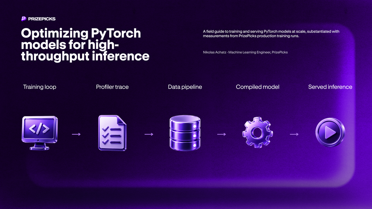
At PrizePicks, model performance is a user experience problem. Every delay in training, scoring, or serving can affect how quickly we respond to new information and how snappy the app feels in the moments that matter. This article shows how we approach that problem: profile before optimizing, separate data bottlenecks from model bottlenecks, and make serving paths faster with techniques like better data loading, mixed precision, model compilation, and inference-only execution. The goal is not optimization for its own sake, but building systems that keep predictions fast, reliable, and ready for production.
Contents
- Introduction
- Opinionated PyTorch:
nn.Moduleas structure - Monitoring with the PyTorch profiler
- Data bottlenecks
- Feed the accelerator before you tune the model
- Compile once, cast to bfloat16, and skip autograd at serving time
- Case study: a hidden latency regression
- Takeaways
- References
Introduction
PyTorch performance work admits two distinct objectives: training throughput, measured as wall-clock time to convergence, and inference latency, the per-request service time under a fixed budget. The corresponding optimizations partially overlap but act at different points in the model lifecycle, so we treat them separately. The measurements reported here come from a model my team at PrizePicks trains and serves online: a compact regression network queried synchronously on a latency-sensitive request path and retrained on a regular cadence.
One principle governs the remainder of this work: profile before optimizing. Training slowdowns are typically input-pipeline bound rather than compute bound, and inference latency is more often dominated by kernel-launch and memory-transfer overhead than by arithmetic throughput.
Opinionated PyTorch: nn.Module as structure
Before getting into performance tuning, it helps to make the model code itself easier to reason about. At PrizePicks, we prefer a consistent structure for numerical components, even when they do not contain learned parameters. That consistency makes components easier to test, move between devices, serialize, and inspect in profiling tools. In PyTorch, nn.Module gives us that structure. It becomes less about whether an object has parameters and more about whether it behaves like the rest of the model system.
We implement numerical components as torch.nn.Module subclasses even when they carry no learned parameters and the hot path is pure NumPy. The base class is a structural contract, not a mere parameter container: it imposes one construction and call convention on every component, whether or not that component trains. The concrete payoffs follow.
Consider a representative case: a Halton estimator of the multivariate-normal CDF. It draws a low-discrepancy Halton sequence to integrate the density, is fully deterministic, and carries no learned parameters. It nonetheless subclasses nn.Module:
class HaltonSimulation(nn.Module):
    def __init__(self, dimension, num_samples=2000, seed=42):
        super().__init__()
        # Precomputed constants ride along as buffers. They move
        # with .to(device), serialize with state_dict, and show up
        # under the module's name in a profiler trace.
        self.register_buffer("sqrt_2", torch.sqrt(torch.tensor(2.0)))
        self.register_buffer("base_samples", self._draw_halton(dimension, num_samples, seed))

    @torch.no_grad()
    def forward(self, mean):
        # One entry point dispatches to a NumPy path or a torch path.
        if isinstance(mean, np.ndarray):
            return self._forward_cpu(mean)   # pure NumPy
        return self._forward_gpu(mean)       # torch tensors
What the base class buys:
- Single entry point.
forwardis the sole call surface. Precomputed state, comprising the sample matrix and derived constants, is registered throughregister_bufferrather than stashed in module globals or closure state, so the object fully specifies its own inputs.
- Device placement and serialization.
- Registered buffers migrate with
.to(device)and serialize throughstate_dict()with no additional code. A free-function implementation would reimplement both mechanisms by hand.
- Registered buffers migrate with
- Testability.
- A test constructs the module at reduced dimension, invokes
forward, and asserts on the return. Because buffers are attributes, the precomputed state is directly inspectable, and the single call surface bounds the test matrix.
- A test constructs the module at reduced dimension, invokes
- Fixed interface for a GPU path.
- The
forwardsignature is stable, so a tensor backend slots into_forward_gpuwith no caller changes. The NumPy path ships first, and the accelerated path is strictly additive.
- The
- Profiler attribution.
- An
nn.Moduleregisters a named scope in the trace. Even a NumPy-onlyforwardis attributed toHaltonSimulationrather than folded into an anonymous frame, so its cost is isolable against the remainder of the model.
- An
The overhead is a single super().__init__() call. In exchange, every numerical component in the codebase exposes uniform construction, state ownership, device handling, and profiler attribution, learned or not.Monitoring with the PyTorch profiler
Optimization work gets expensive when it starts with guesses. Profiling gives us a shared source of truth: are we waiting on data, spending time in the model, paying memory-transfer costs, or seeing overhead from the serving path? For this work, torch.profiler gave us that view across CPU and accelerator activity. Rather than trace every step, we capture a steady-state window so the data is small enough to inspect and clean enough to trust.
torch.profiler instruments CPU and CUDA activity, recording per-operator timing, allocation, and call stacks. Its practical utility inside a training loop hinges on the schedule parameter. Rather than tracing from the cold start, one samples a fixed window of steps at steady state, which bounds trace size and excludes warmup artifacts from the measurement.
from torch.profiler import profile, schedule, ProfilerActivity, tensorboard_trace_handler

with profile(
    activities=[ProfilerActivity.CPU, ProfilerActivity.CUDA],
    schedule=schedule(wait=1, warmup=1, active=3, repeat=1),  # skip 1, warm 1, record 3
    on_trace_ready=tensorboard_trace_handler("./profiler"),
    record_shapes=True,
    profile_memory=True,
    with_stack=True,
) as prof:
    for batch in loader:
        train_step(batch)
        prof.step()  # advances the schedule each iteration
schedule(wait, warmup, active)skipswaitsteps, warms caches and compilation overwarmupsteps, then capturesactivesteps. Tracing every step inflates the file and contaminates the timings with warmup transients.record_shapes,profile_memoryattribute latency and allocation per operator and per input shape, which isolates the dominant kernel and establishes whether the run is memory bound.with_stackretains the Python call stacks, mapping each kernel back to its originating source line.tensorboard_trace_handleremits a TensorBoard-readable trace. For a terminal summary,prof.key_averages().table(sort_by="cuda_time_total", row_limit=20)ranks operators by aggregate CUDA time.
The profiler is gated to fire once per job, on the accelerator device only. The resulting trace is the primary artifact for any throughput regression, and it settles the compute-bound versus input-bound question on which the next section turns.
Data bottlenecks
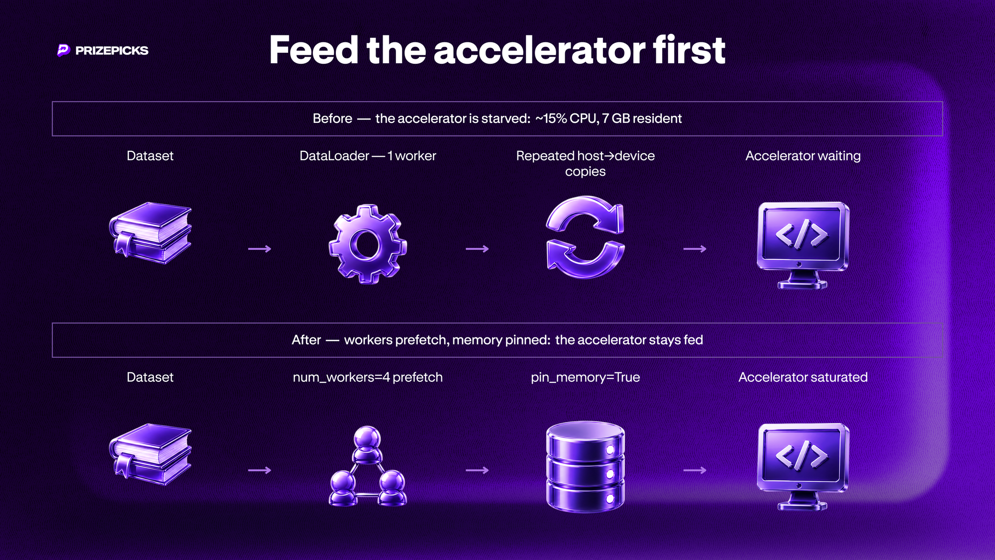
The first question in performance work is often simple: who is waiting on whom? A model may look slow from the outside, but the accelerator may actually be idle while the data pipeline catches up. In one production training run, memory plateaued around 7 GB while CPU utilization stayed low. That pushed the investigation away from model arithmetic and toward the input path: how batches were loaded, transferred, and made available to the accelerator.
The binding constraint must be identified before optimization begins, and the reflexive assumption of accelerator saturation is usually wrong. The trace below is drawn from a production training run: resident memory ramps to roughly 7 GB and plateaus, while CPU utilization holds near 15% for the duration.
Resource usage during training: memory ~7GB, CPU ~15%
Resource trace for one training run. Resident memory plateaus near 7 GB, while CPU utilization holds at a 15% median.
A compute-bound run saturates the CPU or GPU near 100%. At 15%, the process was not spending its time on arithmetic. That pointed us toward the input path rather than the model itself, and the remedy belonged in the DataLoader, through worker count and prefetching, not in a larger accelerator.
To confirm, instrument per-step data-fetch latency against forward-pass latency and read device utilization. Low utilization paired with a fetch latency comparable to the compute latency confirms the pipeline as the bottleneck.
Feed the accelerator before you tune the model
Once we know the bottleneck, the optimization choice gets clearer. If the accelerator is waiting on data, tune the data pipeline. If memory bandwidth or numerical precision is the constraint, use mixed precision carefully. If training is unstable, use techniques like gradient clipping and staged training. If serving latency is the issue, remove request-path overhead with compilation and inference-only execution. This gives the reader a decision guide before we get into the PyTorch-specific levers.
Of the five levers below, four are model-side and one is the data pipeline. On our runs the data pipeline dominated all four combined: the same trace that sat at 15% CPU utilization was the single largest recoverable cost, and no amount of mixed precision or optimizer tuning moves a GPU that is waiting for data. The model-side techniques matter, but only once the accelerator is actually fed.
Data pipeline
Three DataLoader parameters, in decreasing order of impact:
num_workers=N: subprocesses that prefetch batches concurrently with GPU compute. Begin atmin(4, cpu_count // 2)and increase while device utilization keeps climbing. The useful ceiling is set by host core count and memory bandwidth, and the exact plateau is workload-dependent enough that it is worth reading off the utilization curve rather than guessing. On our input-bound trace this was the difference between a starved accelerator and a fed one.pin_memory=True: allocates batches in page-locked host memory, enabling faster host-to-device transfer. It is most useful when those transfers can overlap with compute, so it pairs naturally with worker prefetching.persistent_workers=True: retains worker subprocesses across epochs. Without it, workers are re-forked every epoch, and the fork cost dominates short epochs.
DataLoader(dataset, batch_size=128, num_workers=4,
           pin_memory=True, persistent_workers=True)
Mixed precision
Casting the forward pass to a 16-bit dtype halves memory traffic and dispatches to Tensor Cores on Ampere and later architectures. We prefer bfloat16 to float16. BF16 preserves the 8-bit exponent of FP32, and with it the ~1e38 dynamic range, so it obviates the loss scaler and remains numerically well-conditioned across the wide loss-magnitude swings characteristic of staged training.
# bfloat16: no GradScaler needed
with torch.autocast(device_type=device_type, dtype=torch.bfloat16):
    loss = criterion(model(inputs), targets)
FP16, by contrast, carries only a 5-bit exponent (maximum ~65,504) and therefore requires a GradScaler to keep small gradients from flushing to zero. BF16 needs hardware support on Ampere or later (A100, H100) or on Apple Silicon (MPS).
Gradient clipping
Clipping the global gradient norm bounds the update magnitude and prevents a single outlier batch from destabilizing the parameters. The effect is most pronounced at stage transitions, where a newly trainable head emits large gradients before it converges.
torch.nn.utils.clip_grad_norm_(model.parameters(), max_norm=1.0)
optimizer.step()
Optimizer and schedule
We use AdamW in preference to Adam. AdamW applies decoupled weight decay directly to the parameters, whereas Adam folds decay into the adaptive-gradient term and thereby scales regularization inversely with gradient magnitude, an interaction that is almost never intended. The optimizer is paired with CosineAnnealingWarmRestarts, under which the learning rate anneals to a floor over each period and then resets. The restarts inject the periodic perturbation needed to escape the sharp minima in which a monotone schedule would otherwise trap the iterate.
Staged training with parameter freezing
When multiple heads optimize distinct loss terms, joint training lets their gradients interfere through the shared backbone. We instead train the backbone jointly with the first head, freeze it (requires_grad=False), and then fit the second head against the now-frozen representation. Freezing additionally elides the backward pass over the frozen subgraph, so the second phase is cheaper per step.
# Stage 2: freeze backbone, train head only
for p in model.backbone.parameters():
    p.requires_grad = False

# Rebuild the optimizer. Flipping requires_grad does not
# drop params it already registered.
optimizer = AdamW(
    filter(lambda p: p.requires_grad, model.parameters()), lr=lr,
)
One caveat: the optimizer should be rebuilt after freezing. Flipping requires_grad changes the backward pass, but it does not remove those parameters from the optimizer’s param_groups. Reconstructing the optimizer over the trainable subset makes the freeze explicit and prevents stale optimizer state or zero-gradient behavior from keeping frozen parameters in play.
Compile once, cast to bfloat16, and skip autograd at serving time
Training speed helps us iterate. Serving speed affects the user experience directly. Once a model is in production, every avoidable millisecond on the request path matters. The serving optimizations below all have the same goal: do expensive setup once, reduce repeated work, and keep each prediction path as lean as possible.
The following techniques govern serving latency and throughput. Each applies to the trained model at load and call time.
torch.compile with dynamic shapes
torch.compile() traces the model and lowers it to fused kernels through the TorchInductor backend, typically yielding a 20–40% GPU speedup. The mechanism is kernel fusion. In eager execution each operator is a distinct kernel launch that reads its operands from global memory and writes its result back, so a chain of elementwise operators is dominated by memory traffic and launch overhead rather than by arithmetic. Fusion collapses the chain into a single kernel and keeps the intermediates resident in registers, reducing global-memory access to one read at the input and one write at the output. The elementwise ops become memory-bandwidth-free, and the launch overhead amortizes to a single dispatch.
Kernel fusion: eager mode runs each op as a separate kernel with a memory round-trip each time; torch.compile fuses them into one kernel with a single round-trip

Eager execution issues one kernel per operator, incurring a global-memory round-trip between each. torch.compile fuses the operators into a single kernel, holding intermediates in registers and touching global memory only at the boundaries.
When input shapes vary at inference, shape specialization becomes part of the latency budget. The default path may specialize a compiled graph and recompile after shape changes, while dynamic=True asks PyTorch to generate a more shape-flexible graph up front. That tradeoff should be measured on the workload: dynamic compilation avoids some recompiles, but can also increase compilation cost or reduce the quality of a specialization.
# Compile once at load, not per request.
model = torch.compile(model, dynamic=True)  # validate against eager and static compile on your shapes
Compilation should be performed once at startup. It is deferred to the first forward call and costs between hundreds of milliseconds and several seconds, so it must never sit on the request path.
inference_mode over no_grad
On the serving path we use torch.inference_mode() in preference to torch.no_grad(). Both suppress gradient recording, but inference_mode additionally elides autograd’s version-counter and view-tracking bookkeeping, shedding per-operator overhead that no_grad retains. The context is valid for any code path that does not invoke .backward().
with torch.inference_mode():
    output = model(inputs)
Right-sizing the model
Latency scales with parameter count, so the smallest model that attains the accuracy target is the correct serving choice. The figure below plots measured median inference latency against parameter count across 34 training runs.
Inference latency vs. model size across 34 runs
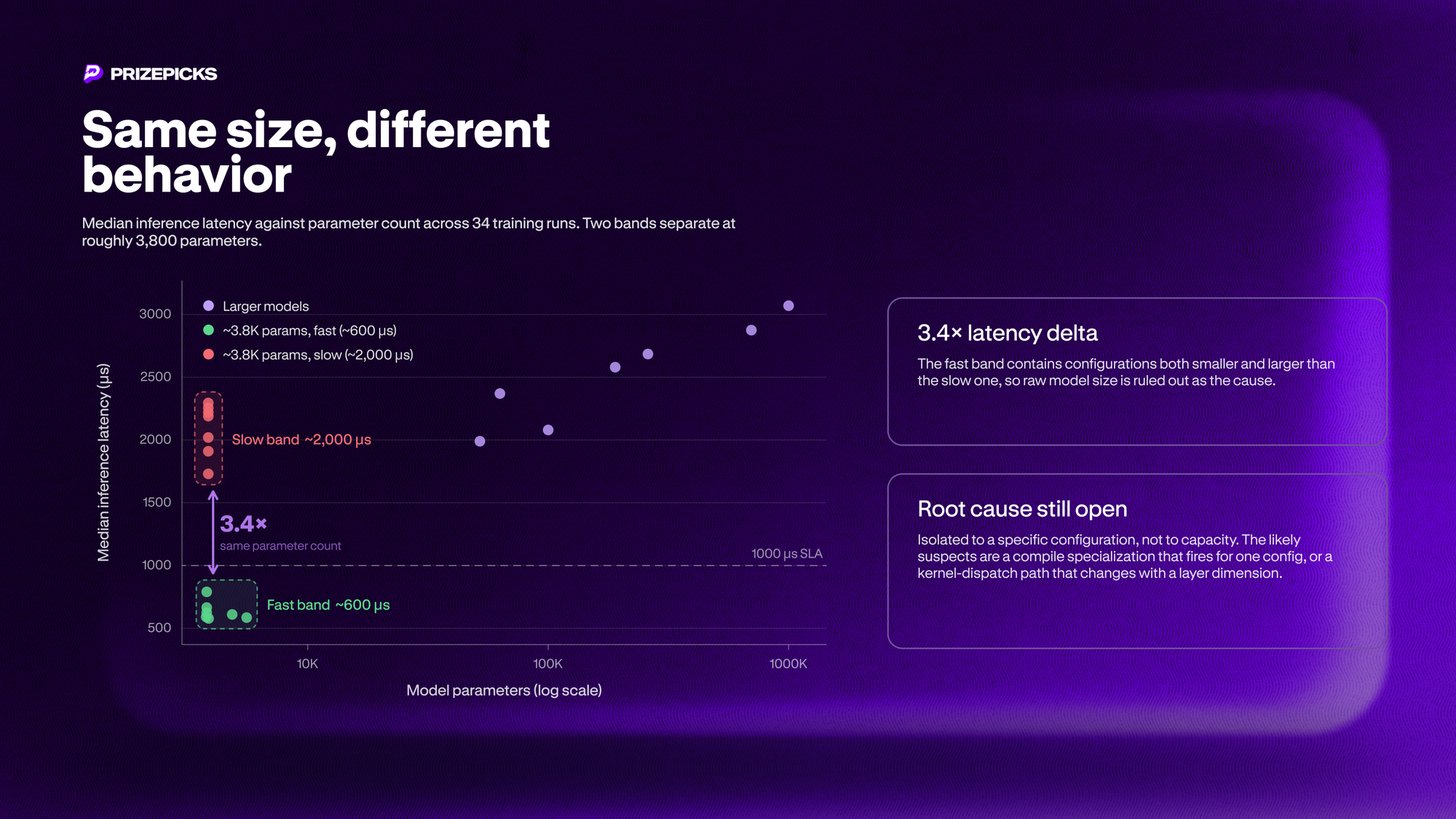
Median inference latency against parameter count, 34 runs. Latency rises with capacity, but two distinct clusters emerge at ~3,800 parameters (analyzed below).
Case study: a hidden latency regression
The most important regressions are not always obvious in a single benchmark. In this case, cross-run latency tracking surfaced a 3.4x slowdown among models that looked nearly identical by size. That is the value of measuring over time: it catches patterns that one-off checks miss. For a production product, that kind of visibility is what keeps performance issues from quietly reaching users.
The latency figure exposes a regression that no single benchmark run could reveal. Among the smallest models, all clustered near 3,800 parameters and drawn from the same architecture family, the measurements bifurcate into two bands:
- Fast band, ~600 us (green), at 3,750–3,870 parameters.
- Slow band, ~2,000 us (red), at a specific 3,858-parameter configuration.
The parameter counts are within a few percent of one another, yet a consistent 3.4× latency delta separates the bands. The delta does not scale with capacity: the fast band includes configurations both smaller and larger than the slow one, so raw size is ruled out as the cause. We have isolated the split to a specific model configuration rather than to model size, but we have not yet root-caused the trigger itself. The logged fields distinguish the two bands only by their outcome, not by the mechanism, and the usual suspects for a step-change of this shape are a compile specialization that fires for one configuration and not the other, or a kernel-dispatch path that changes with a layer dimension. Confirming which would require re-running both configurations under the profiler with identical inputs, which is in progress.
The honest state of this investigation is itself the point. Cross-run latency tracking surfaced a real 3.4× regression that no single benchmark would flag, since each run in isolation satisfies its own threshold. Attribution came second, and it remains unfinished. The value of the instrumentation was making the anomaly impossible to miss in the first place.
Takeaways
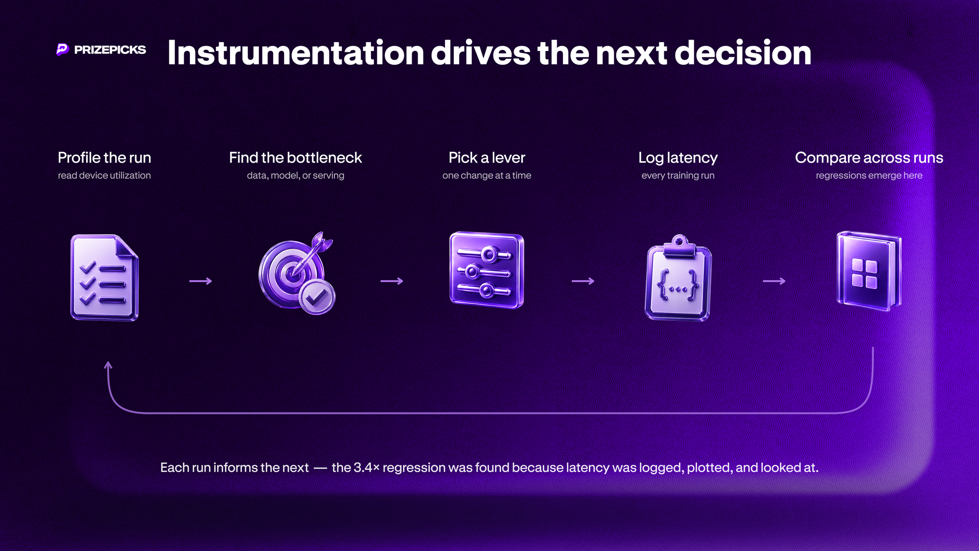
Reduced to a decision procedure, the article is three moves. Before optimizing anything, run the profiler once and read device utilization: if it is low, the accelerator may be starved, and the first fix to test is often in the DataLoader, not the model. Only after the accelerator is fed do the model-side levers pay off, and among them bfloat16 and a measured use of torch.compile are the two with the highest ratio of speedup to risk. And log inference latency on every training run, because the regressions that matter most are invisible in any single run and only emerge across the series.
Everything else in this article is elaboration on those three moves. The 3.4× regression was not found by being clever. It was found because the latency was logged, plotted, and looked at. Instrumentation is the whole discipline. The optimizations are downstream of it.
If you are a free agent looking to get drafted to an Engineering team that solves real world problems like this in-house, explore our open positions below.


References
Compilation
- torch.compiler: overview of the compilation stack (TorchDynamo, TorchInductor).
- torch.compile: API reference, including
dynamicandmode. - Introduction to torch.compile: tutorial covering fusion, graph breaks, and recompilation.
- Dynamic shapes: how symbolic shapes avoid per-shape recompilation.
Profiling
- torch.profiler: API reference for
profile,schedule, and activities. - PyTorch Profiler recipe: schedule, shapes, memory, and stack capture in a loop.
- Profiler with TensorBoard: reading traces and the trace-handler output.
Mixed precision
- torch.amp: automatic mixed precision reference:
autocast,GradScaler, and supported dtypes. - AMP examples: autocast and gradient-scaling usage patterns.
Data loading
- torch.utils.data:
DataLoader,num_workers,pin_memory,persistent_workers.
Optimizers, scheduling, and gradients
- torch.optim.AdamW: decoupled weight decay.
- CosineAnnealingWarmRestarts: cosine annealing with warm restarts.
- clip_grad_norm_: global gradient-norm clipping.
- Loshchilov & Hutter (2019), Decoupled Weight Decay Regularization: the AdamW paper.
- Loshchilov & Hutter (2017), SGDR: Stochastic Gradient Descent with Warm Restarts: the warm-restarts paper.
Modules and inference
- torch.nn.Module: base class, buffers,
state_dict, andto(). - register_buffer: non-parameter persistent state.
- torch.inference_mode: inference-only autograd bypass.